 Journal of Medical Research and Surgery
PROVIDES A UNIQUE PLATFORM TO PUBLISH ORIGINAL RESEARCH AND REMODEL THE KNOWLEDGE IN THE AREA OF MEDICAL AND SURGERY
Journal of Medical Research and Surgery
PROVIDES A UNIQUE PLATFORM TO PUBLISH ORIGINAL RESEARCH AND REMODEL THE KNOWLEDGE IN THE AREA OF MEDICAL AND SURGERY
Journal of Medical Research and Surgery
PROVIDES A UNIQUE PLATFORM TO PUBLISH ORIGINAL RESEARCH AND REMODEL THE KNOWLEDGE IN THE AREA OF MEDICAL AND SURGERY
Journal of Medical Research and Surgery
PROVIDES A UNIQUE PLATFORM TO PUBLISH ORIGINAL RESEARCH AND REMODEL THE KNOWLEDGE IN THE AREA OF MEDICAL AND SURGERY


 Indexed Articles
Select your language of interest to view the total content in your interested language
Bin Zhao1*, Jinming Cao2
1School of Science, Hubei University of Technology, Wuhan, Hubei, China
2School of Information and Mathematics, Yangtze University, Jingzhou, Hubei, China
Correspondence to: Bin Zhao, School of Science, Hubei University of Technology, Wuhan, Hubei, China
Received date: January 25, 2021; Accepted date: February 11, 2021; Published date: February 18, 2021
Citation: Zhao B, Cao J (2021) The Impact of COVID-19 on Farmers’ Economic Income in Hubei Province of China During the COVID-19 Epidemic. J Med Res Surg
2(1): pp. 1-9. doi: 10.52916/jmrs214038
Copyright: ©2021 Zhao B, et al. This is an open-access article distributed under the terms of the Creative Commons Attribution License, which permits unrestricted
use, distribution and reproduction in any medium, provided the original author and source are credited.
This paper discusses the statistical measurement of the impact of COVID-19 major emergencies on farmers’ economic income in Hubei Province. Hubei Province was selected as the object of analysis, and five data of total output value of agriculture, forestry, animal husbandry, fishery and per capita disposable income of farmers in Hubei Province from the first quarter of 2013 to the second quarter of 2020 were collected by using the Internet. Since all the collected data were macroeconomic data, these data were taken the logarithm to meet the economic significance.
The per capita disposable income of farmers was taken as the response variable, and the main factors affecting farmers’ income were obtained by factor analysis. Livestock husbandry and fishery industries were the main industries in Hubei Province. Then the score of factor analysis were taken as explained variable to establish a regression model composed of influencing factors. This paper uses the multiple linear regression, support vector regression to fitting and forecasting data, ARIMA model of time series analysis, introduced at the same time, through the AIC model choice, with the first quarter of 2013 to 2019 in the second quarter fitting training, backward prediction two quarters, and three or four quarter of 2019 compared with the real data, through to the predicted results of the sequence diagram and evaluation index model to compare the mean square error (RMSE).
Three models predict per capita disposable income of farmers in the first and second quarter of 2020. It has been found that performance better ARIMA model in the model compare is worse than before, and three kinds of predicted values are higher than the real value of the model, showed the outbreak to the influence of the agricultural economy in Hubei province is serious. On this basis, taking into account the characteristics of geomorphic climate in Hubei province, constructive suggestions are put forward.
COVID-19, Multiple linear regression, Support vector regression, ARIMA model.
Thanks to the hard work of the whole nation, the epidemic prevention situation in China has been constantly improved, and the order of production and life has been quickly restored. To win the critical period of building a well-off society in all aspects and the decisive battle against poverty, the impact of the COVID-19 epidemic on agriculture and the rural economy should be scientifically studied and judged, and appropriate responses should be made. It is of great significance to ensure the well-being of a well-off society and the quality of poverty alleviation.
The impact of COVID-19 on the agricultural economy mainly includes the impact on the supply of agricultural products, the impact on livestock, poultry and aquaculture, the impact on the supply of agricultural materials and spring tillage preparation, and the impact on the international trade of agricultural products, etc [1,2].
Research on the relationship between agricultural industrial structure and economic growth from the perspective of farmers’ income level: Chen Kai [3] used the grey correlation method to analyze the relationship between rural household operating income and the output value of planting, forestry, animal husbandry and fishery in the Yangtze River Delta region. Yang Zhong-Na, et al. [4] analyzed the impact of agricultural structure and its changes on agricultural growth in southern Xinjiang from 2000 to 2011, and pointed out that agricultural industrial structure has restricted agricultural economic growth, indicating that the relationship between agricultural industrial structure and agricultural economic growth is spatially regional [5-6].
Therefore, it is very important to analyze the impact of the epidemic on the agricultural economy, which can guide the direction of agricultural structural reform.
In this paper, the main income sources of farmers are selected as the analysis indicators, including agriculture, forestry, animal husbandry, and fishery. Some data are shown in Figure 1.
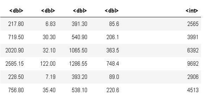 Figure 1: Partial data diagram.
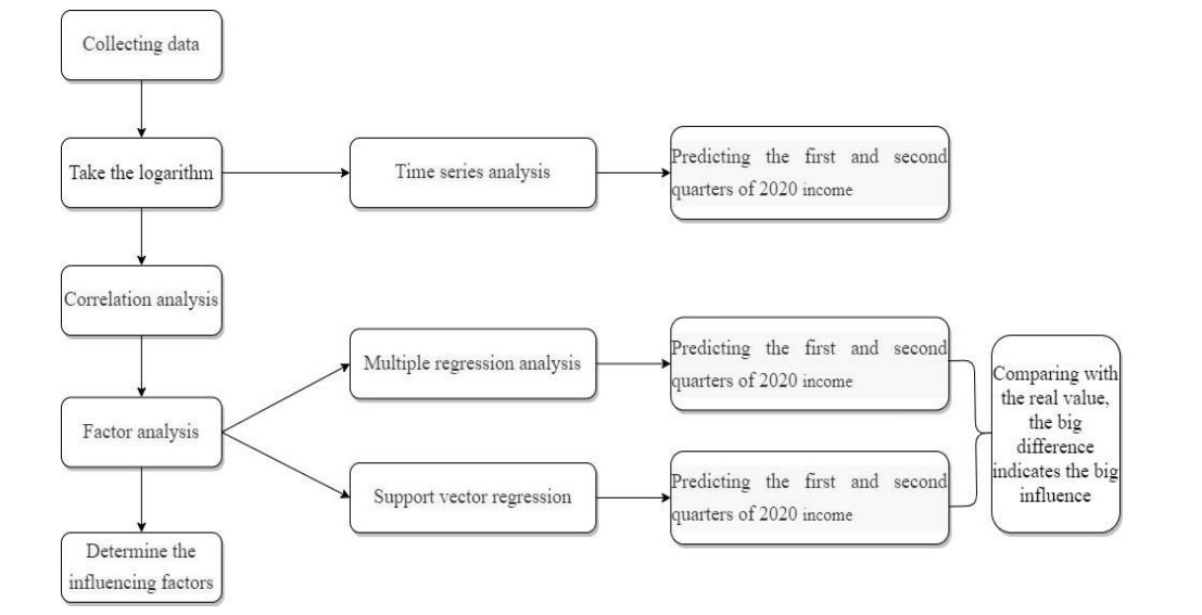
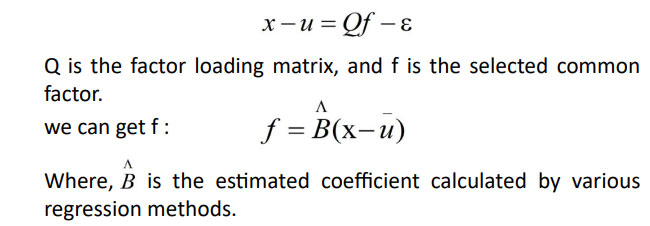
variables hidden among observable variables. Therefore, this paper selects the method of factor analysis to analyze the common factors affecting per capita disposable income, and constructs new variables according to the factor score, to eliminate the impact of the correlation of original data. For the 5 variables of the total output value of agriculture, forestry, animal husbandry and fishery and per capita disposable income of rural residents, we used the principal component method to conduct factor analysis:
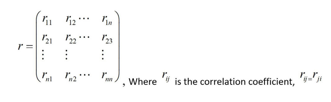
Spearman correlation coefficient analysis of pre-data calculation in Hubei province was conducted in this paper, and the correlation coefficient matrix was visualized. The results are shown in Figure 2.
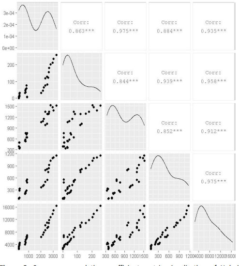 Figure 2: Spearman correlation coefficient matrix visualization of Hubei
Province.
Figure 2: Spearman correlation coefficient matrix visualization of Hubei
Province.As can be seen from Figure 2, there is a strong correlation between all variables, with a correlation coefficient above 0.8 showing a strong correlation. Therefore, factor analysis is considered in this paper to eliminate the correlation between variables. KMO test and Bartlett spherical test were performed on the data and the test results were shown in Table 1.
Table 1: KMO and Bartlett tests
| KMO | 0.77 |
| Bartlett test of sphericity | < 0.01 |
As can be seen from Table 1, the KMO value of the data test is greater than 0.5, and the P-value of bartlett’s spherical test is less than 0.05. Therefore, the test results can be considered as applicable to factor analysis.
The R programming language was used to draw a parallel gravel diagram (Figure 3) to determine the number of common factors. In Figure 4, we drew the gravel diagram for principal
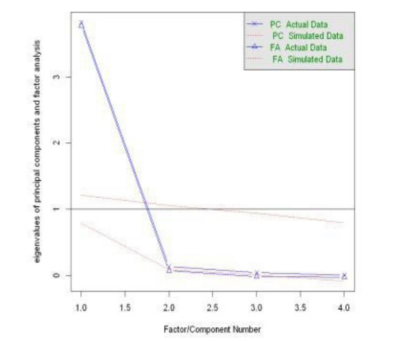 Figure 3: Factor analysis of parallel lithotripsy in Hubei Province.
component analysis for comparison. If PCA principal component analysis was used in the diagram, the number of principal components to be selected from the PC curve was 1. According to the FA curve, the first two eigenvalues are above the corner and are greater than the mean value of the eigenvalues of the simulated data matrix 100 times. Therefore, according to The Kaiser-Harris principle and the parallel analysis criteria, it can be considered that two common factors can be selected for factor analysis.
We determined that it was appropriate to select two common factors, and then carried out factor rotation on the data of Hubei Province, and drew an oblique rotation factor result chart to determine the influencing factors represented by each factor. It can be concluded from Figure 4 that factor 1 represents the driving factor of animal husbandry and factor 2 represents the driving factor of the fishery
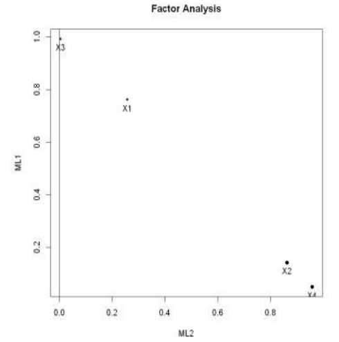 Figure 4: Two-factor figure.
Regression methods can reflect the functional relationship between independent variables and dependent variables, while linear regression assumes that the functional relationship between independent variables and dependent variables is a linear functional relationship, dependent variables can be expressed as a linear combination of independent variables, and the regression of multiple independent variables becomes multiple regression. The choice of linear regression is because the model is simple, intuitive and easy to calculate. The common method of model parameter estimation is the least-squares regression estimation method to minimize the loss function. The linear regression model is expressed as:
y x = + β ε
The results of the factor score table are shown in Table 2.
Table 2: Factor score table of Hubei Province.
| Factor1 | Factor2 | |
|---|---|---|
| x1 | -0.005 | 0.517 |
| x2 | 0.193 | 0.015 |
| x3 | -0.076 | 0.566 |
The corresponding expressions of the two factors can be obtained by converting the data in Table 2 into the factor score function:
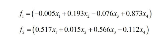
According to the information in Table 2, the common factor 1 represents the animal husbandry driving factor; Common factor 2 represents the fishery driving factor. According to the above analysis, it can be known that for Hubei Province, the main influencing factors of agricultural structure adjustment on farmers’ income include driving the overall economic development led by animal husbandry and vigorously developing animal husbandry, among which the first influencing factor is the most important.
After finding common factors through factor analysis and dimensionality reduction of the original data set, the multiple linear regression model of per capita disposable income of farmers and two common factors was established by using the multiple linear regression method.
In this paper, R language programming was used to carry out multiple regression modeling of farmers’ income and its two common factors in Hubei Province, and the regression equation was obtained as follows:
y=0.36F1+0.29f1+4.90
The R square test can judge the degree of interpretation of independent variables to dependent variables. The closer R square is to 1, the greater the degree of interpretation of independent variables to dependent variables will be. It is known from Table 3 that the common factors of the multiple regression model have a good interpretation of farmers’ income.
Table 3: R squared test value
| Province | R squared |
| Hubei | 0.9584 |
The DW test is used to test the independence between the observed values. The closer the VALUE of the DW test is to 2, the more independent the observed values are. As shown by the table, the value of the common factor of the multiple regression model is close to 2, so it can be considered that the common factor has good independence (Table 4).
Table 4: : RDW test value.
| Province | P-value |
| Hubei | < 0.01 |
F test is a test method to determine whether there is a linear relationship between independent variables and dependent variables. When the P-value of the F test is less than 0.05, it is considered that there is a linear relationship between agriculture, forestry, animal husbandry, fishing, and farmers’ income. It can be seen from the table that the P-value of the F test is far less than 0.05, and it can be considered that there is a linear correlation between the common factor of the multiple linear model and farmers’ income (Table 5).
| Province | DW |
| Hubei | 1.4695 |
If there is a correlation between independent variables, the model is considered to have multiple common linearity. In this paper, the VIF index is selected to test whether there is multicollinearity among independent variables. When the VIF value is less than 10, it can be considered that there is no multicollinearity among independent variables in this multiple regression model. It is known from the table that the VIF test values of the linear model are all less than 10, so it can be considered that there is no multicollinearity between the common factors selected in Factor analysis (Table 6).
| Province | VIF |
| Hubei | 3.48 |
To study the impact of the epidemic on agricultural economic income, we used the historical data from 2013 to 2019 to establish a multiple linear regression model, and used this model to predict the economic income of farmers in the first and second quarters of 2020, and compared and analyzed the predicted data with the actual data, to analyze the impact of the epidemic on farmers. We use the mean square error (Table 7)
Table 7: Linear regression analysis for the first two quarters of 2020.
| Province | Forecast for the first quarter of 2020 | Real value for the first quarter of 2020 | Forecast for the 2nd quarter of 2020 | Real value for the 2nd quarter of 2020 | RMSE |
| Hubei | 8.32 | 8.31 | 8.86 | 8.76 | 0.072 |
It can be seen from the table that the predicted value of Hubei Province in the first and second quarters of 2020 is higher than the true value based on the time series prediction of the data from 2013 to 2019 without the influence of epidemic as the observed value, indicating that the epidemic has a relatively large impact on the disposable income of farmers in Hubei Province, and the epidemic will reduce the economic income of farmers.
The time sequence diagram of model comparison and prediction is shown in Figure 5:
 Figure 5: Comparison and prediction sequence diagram of multiple linear regression models; (a): Comparison time series; (b): Forecast time series.
It can be seen from Figure 5 that the predicted value in the third and fourth quarters of 2019 in Hubei Province is lower than the real value, indicating that the farmers’ income is rising steadily, while the predicted value in the first and second quarters of 2020 is higher than the real value, indicating that the rural economy in these two quarters is seriously affected by the epidemic.
Support vector regression
Model Building
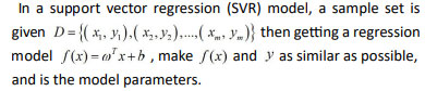
For samples (x,y), traditional regression models usually calculate the loss based on the difference between model output f(x) and real value y. The loss is zero if and only if f(x) and y are exactly equal. On the contrary, The SVR model assumes that we can tolerate an error of ε at most between f(x) and y, and the loss is calculated only when the absolute value of the difference between f(x) and y is greater than ε [7]. As shown in Figure 6 below,
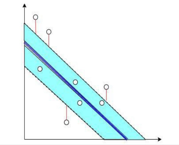 Figure 6: Support vector regression diagram.
w, the points inside the blue strip have no loss, while the points outside have a loss, and the loss is the length of the red line.
First used in the first quarter of 2013 to 2019 in the second quarter fitting training, backward prediction two quarters, and three or four quarter of 2019 compared with the real data, compared with other models, in the first quarter of 2013 to 2019 in the fourth quarter of data forecast in 2020 first and second quarters, to examine the rationality of the model, analyze each model of residual error as shown in figure 7, six models are reasonable.
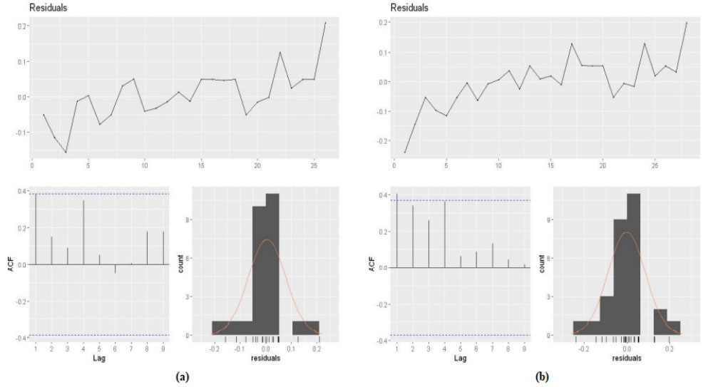 Figure 7: Model comparison with forecast residual graph; (a): Model comparison residuals; (b): The model predicts residuals.
Analysis and interpretation of model results
The time sequence diagram of model comparison and prediction is shown in Figure 8.
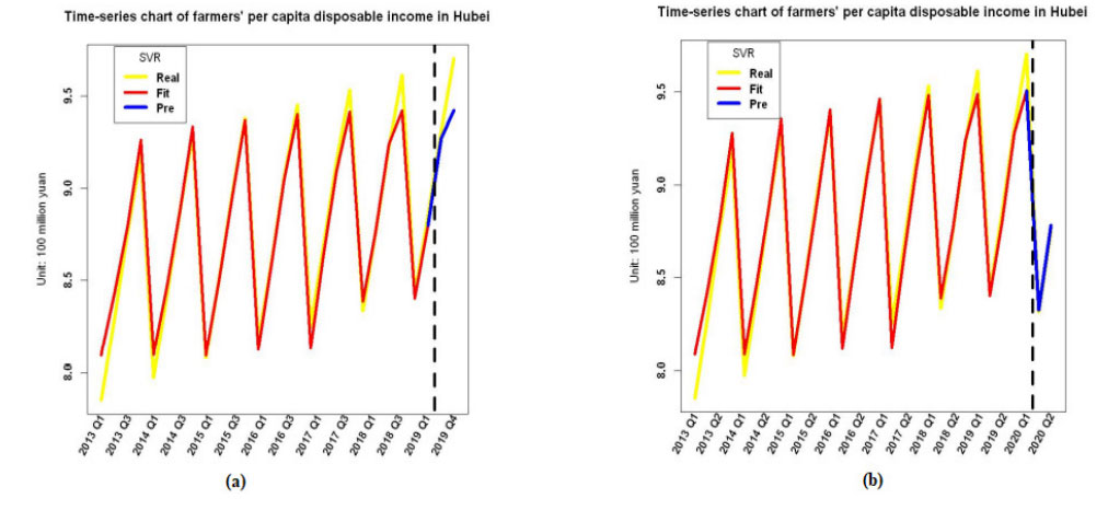 Figure 8: Comparison and prediction sequence diagram of SVR models; (a): Comparison time series; (b): Forecast time series.
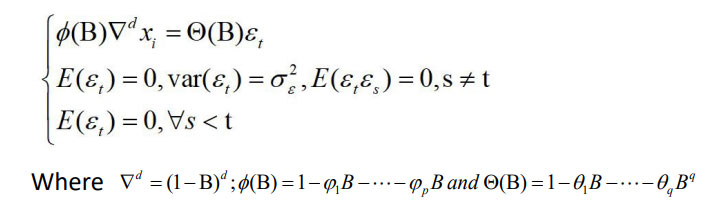
respectively represent the autoregressive coefficient polynomial and the moving smoothing coefficient polynomial of the stationary reversible time series model.
Before establishing the ARIMA model, we first determine the order of the model, i.e., the values of P and Q, and select the appropriate order to achieve the relative optimization of the final fitting model. In the time series model, it is necessary to order the model, and we generally use the AIC criterion and BIC criterion. Where AIC is the weighting function: AIC=-2ln(L)+2K. To achieve the optimal model, we should try to choose the minimum AIC value. In this paper, we use the data from the first and second quarters of 2013 to 2019 to build the ARIMA model, and then predict the per capita disposable income in the first and second quarters of 2020 and compare it with the real value.
Solution and test
After the establishment of the model, it is necessary to evaluate the established time series model. First, we need to test the fitting effect of the time series model through the stationary R-square. Then the white noise test was carried out for the residuals. We can use Q-test to determine whether the residual is white noise. Based on time series analysis, in this paper, the farmers of disposable income, the integrated test, first of all to log processing of raw data, then a stabilized and zero mean treatment of the ARIMA model was established, and one-quarter of Hubei province in 2020 to predict the disposable income of farmers, analyzes the influence of the outbreak. The null hypothesis of the Q-test is: 01 2 : 0 H ρρ ρ = =⋅⋅⋅ =s and the alternative hypothesis is: 1 : (i 1, 2,..,s) H one of ρi = is non-zero at least. Under the condition that the null hypothesisH0 is established, the statistics 2 2 1 (T 2) ~ X s k s n k r Q T T k − = = + − ∑ established. Where T is the number of samples, n denotes the number of positional parameters in the model. When The p-value obtained by the Q-test is less than 0.05, the null hypothesis is rejected. It is believed that the model does not fully recognize the data. If a p-value is greater than 0.05, the model is accepted as recognizing the data well. Also, we made ACF and PACF graphs of residuals to judge whether the residuals are white noise. If ACF and PACF of each order are less than the critical value of the test, the residual is considered to be white noise, that is, the model identifies the data well. Otherwise, it is considered that the model is not fully identified. The result is shown in Figure 9:
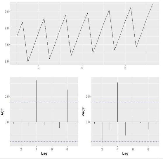 Figure 9: Peasant per capita disposable income time series model residuals
ACF and PACF.
Figure 9: Peasant per capita disposable income time series model residuals
ACF and PACF.By analyzing the ACF and PACF graphs of the time-series model residuals corresponding to all variables in Hubei Province, it can be found that they are all less than the critical value of the test. Therefore, the residuals can be considered as white noise. That is to say, the model obtained in this paper can identify our data well. So we can accept these temporal models.
Through the obtained time series model, we can predict the per capita disposable income. Figure 10 below shows the time series diagram of the per capita disposable income of farmers in Hubei Province.
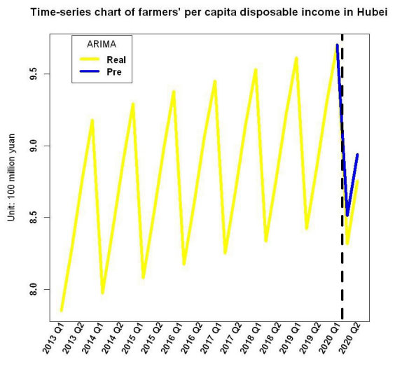 Figure 10: Timing chart of farmers’ per capita disposable income.
It can be seen from Figure 10 that the predicted value of Hubei Province in the first and second quarters of 2020 is higher than the true value based on the time series prediction based on the data from 2013 to 2019 without the impact of the epidemic, indicating that the epidemic has a relatively large impact on the disposable income of farmers in Hubei Province.
The mean square errors of comparison and prediction of all models are shown in Table 8 below.
Table 8:RMSE comparison table for each model.
| Province | ARIME | LM | SVR | |
|---|---|---|---|---|
| Comparison | Hubei | 0.002 | 0.179 | 0.202 |
| Prediction | Hubei | 0.192 | 0.072 | 0.018 |
As can be seen from Table 8, in comparison and prediction of Hubei Province, the performance of the ARIMA model which performed better before is worse than before, and the predicted values of the four models are all higher than the real values, indicating that the income of farmers in Hubei Province is seriously affected by the epidemic.
Based on the modeling and analysis in this paper, we successively put forward suggestions on the impact of agricultural structure adjustment on farmers’ income in Hubei Province.
1. Strengthen macro-control Although we strongly advocate market agriculture and emphasize the dominant position of farmers in the adjustment of agricultural industrial structure, the government should strengthen macro-control in the face of poor income increase of farmers and excessive pursuit of immediate interests, which impair industrial adjustment. In the process of adjusting agricultural industrial structure in Hubei Province, all the work should be carried out with increasing farmers’ income as the goal, to support farmers’ business activities under the industrial structure adjustment as much as possible, and actively play the function of macro-control.
2. Develop aquaculture vigorously The low proportion of aquaculture in the primary industry is an important manifestation of the irrational agricultural industrial structure. Hubei province has rich water resources and unique advantages for aquaculture, but the proportion of fishery in the agricultural industry in Hubei province is only higher than forestry. Therefore, we should pay more attention to aquaculture and vigorously develop aquaculture with local characteristics, such as crayfish in Qianjiang and crab in Xianning, to make it the key point to promote farmers’ income.
3. Strengthen scientific training Local governments and agricultural departments should stick to the central idea of “developing agriculture through science and technology”, persist in improving farmers’ quality through “science and technology training” as a media platform, and help farmers solve various technical problems they may encounter in production, to improve farmers’ agricultural planting techniques. Through the combination of “centralized teaching, on-site teaching and individual guidance”, the innovative mode of agricultural cultivation is promoted, and the prevention and control analysis of possible insect disease disasters is carried out so that farmers can quickly master skills. The government’s science and technology training platform plays an important role in strengthening farmers and radiating the surrounding economic development.
4. Agricultural Economy Combined with China’s special rural conditions, coupled with the lack of implementation of relevant national benefits to farmers, their own land, lack of funds, single information channels, resulting in farmers in the process of agricultural industrial structure adjustment in the face of the market alone in the case of higher costs, limit the increase of income level. In the face of this situation, it is very important to gradually develop a new form of cooperative organization to help the separated and independent farmers establish connections with the large market.

